Frontier-scale RL with Kimi K3

Kimi K3, with just shy of 3T parameters, pushes performance of open weight base models closer to the frontier. At such a large scale, we needed to re-architect portions of our stack to ensure that we could train with high efficiency. Full fine-tuning support for Kimi places an extraordinary amount of stress on our training, communication, and storage systems.

In this blog post, we'll share some of the improvements we implemented to train Kimi cheaply and efficiently. All of these optimizations are live when you fine-tune Kimi K3 on AC2.

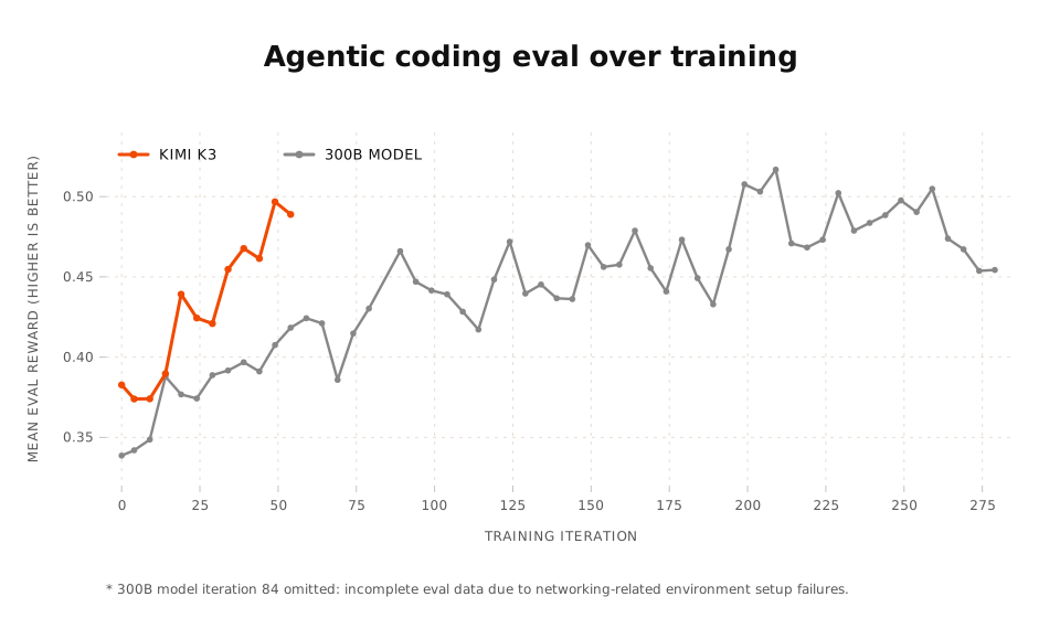
To derisk our implementation, we trained a coding agent using Kimi K3 as the base on a challenging long-horizon task. After 50 steps of training completed within a day, we matched the performance that a smaller 300B-class model reached in multiple days. Empirically, we observe a general trend where larger models tend to have higher slope on new tasks.

Memory management

The primary challenge in large-scale model training is the sheer amount of data that needs to be stored and transmitted during the run. This data is shuttled between the host and device, and falls into two main classes.

Parameter-shaped (scales with model size):

• Model weights: bf16 model weights used in the training engine (GPU memory)
• Adam optimizer state (offloaded to host memory)
  • fp32 master weights
  • Two sets of bf16 moments
  • fp32 gradient buffer

Context-shaped (scales with number of tokens):

• Activations
• Logits
• Routing tensors

When processing large amount of data during training, we can stream data to greatly reduce memory peaks. We outline two such use cases of streaming which provided significant memory savings for Kimi K3: one mitigates the memory footprint of the context-shaped data on the GPU, and the other reduces the parameter-shaped memory usage on the host. In tandem, these optimizations let us reduce the number of GPUs required per training replica by ~40% with minimal latency cost.

Streaming activations

The naive implementation of SiTU looks something like this:

def situ_and_mul(
    x: torch.Tensor,
    beta: float = 4.0,
    linear_beta: float = 25.0,
) -> torch.Tensor:
    gate, linear = torch.chunk(x.float(), 2, dim=-1)
    gate = beta * tanh(gate/beta) * sigmoid(gate)
    linear = linear_beta * tanh(linear/linear_beta)
    return (gate * linear).to(x.dtype)

This implementation is simple but causes the PyTorch's autograd engine to save 6 fp32 copies of the full [R, H] tensor from the forward pass to use in the backward pass. See below for a breakdown of where these saved tensors come from.

Here, R is the number of tokens on the GPU times 16 (the number of routed experts for Kimi K3) and H is the hidden dimension (3072 for Kimi K3). For ~100k tokens per GPU, this results in >100GB of HBM!

To alleviate the memory peak from the unoptimized PyTorch autograd, we implemented a custom operator for SiTU-GLU which

1. Drops all tensors except for the bf16 input tensor x from memory, incurring a small recompute cost for the tanh and sigmoid functions in the backward pass.
2. Streams over the bf16 input tensor and works on a constant sized fp32 workspace for both the forward and backward passes. This works because the activation function is applied element-wise.

With these optimizations, we only need to save the input x, which is a bf16 [R, 2H] tensor. This is only 1/6 of the size of the naive approach, and saves about 90GB of HBM per GPU! Since each B300 has about 270GB of HBM, this saves about 33% of the total memory from each GPU.

Streaming gradients

The Adam optimizer state for large models is partially offloaded to host RAM, since we don’t have enough space on GPU HBM. For gradient updates, we need to transfer gradients computed on device to the host where optimizer state lives in order to update the master weights and moments.

Existing solutions do one big D2H (Device to Host) transfer, update the weights and moments, and send updated model weights back to the GPUs to update the working weights.

However, this materializes a whole extra parameter-shaped fp32 gradient buffer in the CPU. By applying Adam update in chunks, we can essentially eliminate all memory cost of the transfer while not sacrificing performance. This is possible because Adam updates each parameter independently!

Note that the total computation cost is the same in both cases, but streaming adds some communication overhead; since the bottleneck for the update is primarily the optimizer step, the performance degradation is minimal. However, by interleaving transfers with chunked optimizer updates, we can reduce host memory by 4 bytes per parameter. There were originally 12 bytes per parameter, so this is a ~33% reduction! Since we still need the buffer, the savings are slightly reduced.

Sampling performance

Low precision (MXFP4) rollouts

Low precision rollout engines are ideal for two reasons. First, MXFP4 inference engines can run performantly on just 2 B300 nodes (and even fit in just 1 node), whereas a bf16 engine would require 4 nodes. The reduced node count lowers communication volumes over slower scale-out networks (e.g., InfiniBand or RoCE) during inference. Second, since production serving tends to use quantized weights for performance reasons, there is no train-test mismatch related to numerics.

In our training runs, we found that the KL divergence between a bf16 Kimi K3 training forward pass and a bf16 Kimi K3 inference engine was approximately the same as the mismatch between a bf16 Kimi K3 trainer and an MXFP4 Kimi K3 inference engine (W4A8 for the MoE layers, with attention compute and storage in bf16). We hypothesize that the mismatch induced by low precision rollouts against a bf16 training engine is smaller for Kimi K3 relative to other models because the fraction of active parameters stored in low precision for each token is only 47% (about 49B of the 104B active). The fraction of low precision active parameters being this small can be attributed to:

• 3/4 of the model’s layers are KDA layers with parameters in bf16 (over a small fp32 state), and
• everything besides the routed experts are in bf16.

For reference, we can compare this to another popular model, GLM 5.2/5.3, where the shared experts, attention projections, and DSA indexer projections are also all in low precision. GLM 5.2/5.3 ends up having about 97% of the active parameters for each token being low precision.

Weight transfer

Transferring Kimi K3 weights has one quirk that was silently corrupting our rollouts.

Kimi uses Block Attention Residuals (AttnRes), which is a way for tokens to attend to versions of themselves from previous layers. Each candidate $v$ (e.g. previous layer representation of the token) is given a score $s$ via this formula involving a projection weight vector $w$ and norm weight vector $\gamma$ (which are parameters of the model):

where $\odot$ represents elementwise multiplication. The candidates are then combined via softmax weights computed from the scores. We can see from the formula that the projection and norm weights can be multiplied elementwise ($w\odot\gamma$), cached, and reused for scoring all future candidates. This is an optimization that inference engines like SGLang eagerly do on initial weight load.

However, this set of cached weights goes stale during online weight transfers during RL! Therefore, we must recompute it for each AttnRes layer during every weight transfer.

Checkpoint management

A full training checkpoint for Kimi K3 comes out to around 28 TB. We've observed that writing to shared filesystems had an aggregate throughput maxed out at 5–6 GB/s, so saving a 28 TB checkpoint would cost ~75-90 minutes. We've seen significant speed and memory improvements by skipping Linux CPU page caches through the O_DIRECT⌝ flag when writing checkpoints.

The standard path for writing data to the filesystem goes through the page cache. The page cache keeps recently written data in host memory for faster retrieval (https://kernel-internals.org/mm/page-cache/⌝). However, since checkpoints are written once and not re-read shortly after, the page cache doesn’t buy us anything in this case and slows down writes. So, bypassing it is a free speed improvement.

We added an O_DIRECT storage writer for PyTorch distributed checkpointing, a drop-in replacement for the stock filesystem writer. The new writer moves each checkpoint shard through aligned buffers straight to the filesystem, skipping the page cache entirely.

For the same job on identical nodes:

Replacing the buffered saves with O_DIRECT also relieves some of the host memory footprint of the job. A buffered save leaves behind a page-cache footprint that grows with the checkpoint, and it stacks with every retained checkpoint. The O_DIRECT writer's footprint is a fixed amount, independent of checkpoint size.

Trickle-down improvements

Scaling to multi-trillion parameter models exposes new unoptimized areas in our RL stack and infrastructure. Through the process of bringing Kimi K3 training into the platform, we have found new improvements to manage memory, performance, and communication. Many of these improvements generalize beyond just Kimi K3 and further increase the efficiency for all of our existing models as well! If you are intrigued by the different aspects of a complex RL system, you should reach out to us⌝.

Acknowledgements

We thank Moonshot for their contributions to the open source community, including the release of the Kimi K3 model weights as well as the publication of the technical report.